Bayesianity

Assuming that we want a theory of rationality…
1. Desiderata
Interactive: What do we want from a theory of science? Epistemology more generally? Rationality more generally?
(Let them speak for 10 mins. They know but they won’t know the terminology)
Coherence (the world is coherent, so our theory should be)
Answer the right goddamn question: \(P(H \mid E)\), “How likely is the hypothesis given the data?”. Confirm hypotheses; degrees of actual confidence about the real question.
- Generality. Be strictly larger than science: Answer any question. Cover all reasoning.
- Handles unique events
- What is the probability that Lincoln will be assassinated?
- What is the probability that Trump will be assassinated?
- Handles inadmissible evidence
- We’d like one theory that covers science, good intuition, and maths and logic.
- Handles unique events
Uncertainty. Always have other hypotheses; always consider how strong the evidence is.
- Quantification
- Degrees of confirmation
- Exactness: specific values
- Exactness: specific uncertainty
- Falsification. Take out the trash
- Just \(LR \to 0\). The “asymmetry of science” to be explained by the asymmetry of available likelihood ratios.
- Better! disconfirmation is not binary
Reproducibility: unlike others, Bayes puts all its judgments into the model.
- Mechanisms for our intuitions
- “Always use all information. It’s always rational to look (at free evidence).”
- “The order of evidence shouldn’t matter.”
- “Experimenter intentions shouldn’t matter”: Bayesian inference is independent of when you stop collecting evidence!
- “surprising evidence confirms a hypothesis more” Lone anomalies can destroy theories.
- Varied evidence confirms more. Different researchers, different fields, different instruments, different models, different statistical frameworks!
- “you can’t reason your way to a predetermined conclusion.” Conservation of expected evidence. capacity for confirmation is purchased with exposure to refutation.
- “Extraordinary claims need extraordinary evidence”. Hume’s maxim. how extraordinary the evidence must be.
- “There’s something wrong with putting 0 on a hypothesis”. Cromwell’s rule
Help us design experiments. Lindley (1956): expected information gain makes it a theory of inquiry (which question to ask), not just belief revision.
- Parsimony. Automatic (marginal likelihood: a model that can fit anything assigns little to any particular dataset - Jefferys & Berger 1992, MacKay) and explicit (complexity-weighted priors; Solomonoff as the limit). No razor axiom (but simplicity enters from our priors, a backdoor).
Finally consider some ultra-ambitious goals for such a theory:
- Convergence guarantees. Intersubjectivity: priors should “wash out”
- Unification of thought and act (not just epistemology, also decision theory). Beliefs are for acting: Savage integrates credence with utility, and Wald’s complete-class theorems say every admissible decision rule is a (limit of) a Bayes rule
- Optimality
- Uniqueness
Full list
Coherence (the world is coherent, so our theory should be)
- synchronic coherence (probabilism)
- diachronic coherence (conditionalisation)
- Sequential coherence (Show: updating on (x₁,x₂) jointly = updating on x₁ then x₂. This coherence under decomposition is special - most ad hoc belief-revision rules fail it.)
Answer the right goddamn question: \(P(H \mid E)\), “How likely is the hypothesis given the data?”. Confirm hypotheses; degrees of actual confidence about the real question.
- Bayesianism is a quantitative confirmation theory: \(E\) confirms \(H\) iff \(P(H \mid E) > P(H)\), i.e. iff \(P(E \mid H) > P(E \mid \neg H)\).
Generality. Be strictly larger than science: Answer any question. Cover all reasoning.
- Handles unique events
- What is the probability that Lincoln was assassinated?
- In 1865, what was the probability that Lincoln will be assassinated?
- What is the probability that Trump will be assassinated?
- What is the probability that the defendant is guilty?
- Not scientific questions, clearly. Bayes works fine.
- We’d like one theory that covers science, intuition, and logic. Classical logic handles certainty; Bayes claims to be its unique extension to uncertainty (Cox: real-valued plausibilities are consistent with propositional logic).
- frequentism is a theory of procedures, not beliefs; falsificationism is qualitative and flees from the commonsensical idea of conformation; formal learning theory is about eventual convergence.
- Big problem: logical uncertainty
- Handles unique events
Uncertainty
Quantification
- Degrees of confirmation
- Exactness: specific values
- Exactness: specific uncertainty
Falsification. Take out the trash
- Just \(LR \to 0\). The “asymmetry of science” to be explained by the asymmetry of available likelihood ratios.
- Better! disconfirmation is not binary
Reproducibility: unlike others, Bayes puts all its judgments into the model.
Mechanisms for our intuitions
- Use all information. Combine information from multiple sources and related phenomena. Use your hunches. It’s always rational to look at free evidence. “Consider all the evidence” and “looking is rational”
- The order of evidence shouldn’t matter.
- Experimenter intentions shouldn’t matter: Bayesian inference is independent of when you stop collecting evidence!
- Likelihood Principle: Inference shouldn’t depend on intentions, past analyses, stopping. In Bayes (and LLism) inference depends on the data only through the likelihood function. Birnbaum (1962) derived it from sufficiency plus conditionality.
- Lone anomalies can destroy theories. “surprising evidence confirms a hypothesis more”
- varied evidence confirms more. Different researchers, different fields, different instruments, different models, different statistical frameworks!
- Replications of the same kind share instruments, auxiliaries, and systematic errors, so they’re highly correlated under the rivals too, so \(LR \approx 1\), a negligible boost to the posterior. Diverse evidence is evidence nearly independent conditional on each rival, so each new kind discriminates against a different chunk of ¬H.
- “you can’t reason your way to a predetermined conclusion.” Conservation of expected evidence. \(\mathbb{E}[\text{posterior}] = \text{prior}\): no experiment can be expected to confirm, and if E would confirm then ¬E must disconfirm. No experiment can confirm under every outcome; capacity for confirmation is purchased with exposure to refutation.
- Qu antitative Hume’s maxim: “Extraordinary claims need extraordinary evidence.” Testimony establishes a miracle only if the testimony’s falsehood would be more improbable than the miracle - i.e. the likelihood ratio must exceed the prior odds against. how extraordinary the evidence must be.
- “There’s something wrong with putting 0 on a hypothesis”. Cromwell’s rule
Help us design experiments. Lindley (1956): expected information gain makes it a theory of inquiry (which question to ask), not just belief revision.
Parsimony. Automatic (marginal likelihood: a model that can fit anything assigns little to any particular dataset - Jefferys & Berger 1992, MacKay) and explicit (complexity-weighted priors; Solomonoff as the limit). No razor axiom (but simplicity enters from our priors, a backdoor).
De Finetti exchangeability.Explains what iid models and “objective chance” talk mean in credence terms, bridge rationality theory and statistical practice (plus Lewis’s Principal Principle for chance–credence coordination).Handle classic puzzles:
- Quantitative answer to the ravens paradox (a non-black non-raven confirms “all ravens are black” - a negligible amount; Hosiasson-Lindenbaum 1940),
- Tames irrelevant conjunction
- Handles Duhem–Quine: blame for a failed prediction is apportioned across theory and auxiliaries by their priors and likelihood contributions (Dorling 1979).
Finally, some ultra-ambitious goals for a theory:
- Optimality (guaranteed convergence to truth, adversarial robustness, epistemic efficiency)
- Intersubjectivity: priors should wash out
- Unification of thought and act (not just epistemology, also decision theory)
- Beliefs are for acting: Savage integrates credence with utility, and Wald’s complete-class theorems say every admissible decision rule is a (limit of) a Bayes rule.
- Uniqueness. The insane claim that no one else can compete with Bayes.
Is there anything that gets us all of these at once?
2. Bug
Imagine you’re a doctor. A patient comes in for a routine screening without symptoms.
- The prevalence of breast cancer in her cohort is 1%.
- Mammogram sensitivity \(P(\text{positive test} \mid \text{has cancer})\): 90%.
- False-positive rate \(P(\text{positive test} \mid \text{no cancer})\): 9%.
- She tests positive.
- What’s the probability she has cancer? \(P(\text{cancer} \mid \text{positive mammogram})\):
Interactive: give them a minute to write. Take a vote.
| Tally of student answers | |
|---|---|
| Not enough info | |
| 1% | |
| 9% | |
| 48% | |
| 91% |
Most will say ~91%. Calculate the correct answer. I will justify this calculation in a moment.
\[P(\text{has cancer} \mid \text{+mamm})\]Who has seen this thing | before? It means “given”, “after”, “assuming”, “having observed”. So P(having cancer assuming that I have tested positive on this weak test).
\[\begin{aligned} P(\text{cancer} \mid \text{+mamm}) &= \frac{P(\text{+mamm} \mid \text{cancer}) \times P(\text{cancer})}{P(\text{+mamm})} \\ &= \frac{0.9 \times 0.01}{0.9 \times 0.01 \,+\, 0.09 \times 0.99} \\ &= \frac{0.009}{0.0981} \\ &\approx 0.09 \end{aligned}\]Yes, 9%: more than nine out of ten positive tests are false alarms. These are real parameter values by the way, for the US right now.
What do doctors answer? The most common answer among them is “90%”. Only around 20% of them get it right. We first tested them on this 50 years ago. It’s pretty famous and they still haven’t improved. This is a horrible bug in human thought!
This test is performed millions of times a year, so consider the downstream costs: we scare millions of women a year and send them for unnecessary biopsies - a giant needle taking a little chunk of your chest. Overdiagnosis, overtreatment, terrified patients. And the people failing here are highly intelligent, caring, and trained for a decade.
Something makes us fail here, and it’s not lack of talent. Humans fail here because we don’t use the equation.
Big fact 1: Intelligence != rationality. smart humans are not automatically rational
2. Equation
Proof
Let $$\Omega$$ be the set of all possible events. Let $$A$$ be some event. Let $$P(A)$$ be its area.
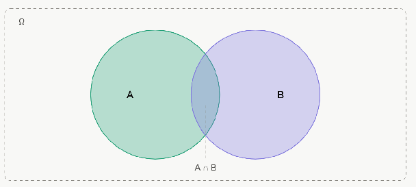
Let $$P(A \mid B)$$ be the area of A that is inside B: the conditional probability of A given B.
We can also read | as "zoom". A zoom B.
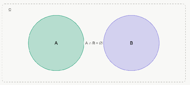
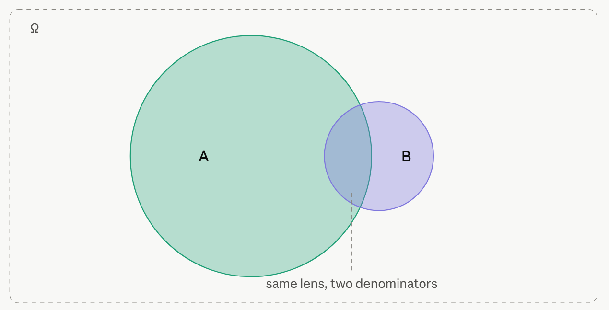
Interactive: what's $$P(A \mid A)$$? It equals 1 — iff $$P(A) > 0$$.
Conditioning means to assume true. It is zooming in such that nothing exists except in B.
I have reduced my uncertainty. If I'm looking in Omega, the whole space, I have maximum uncertainty. If I condition on some event A, I get to ignore everything that isn't in A. Ignore the worlds where ~A.
Big fact 2: To reduce uncertainty is to destroy possibility. To zoom in.
- Among olympiad kids, what fraction are really cool?
Among really cool people, what fraction are olympiad kids? - Among ESPR participants, what fraction are olympiad kids?
Among olympiad kids, what fraction went to ESPR?
We proceed to derive Bayes' theorem from axioms. We grant ourselves set theory. Consider an "event" A with a probability (area) P(A).
The essence of a probability is being about the size of sets, thus nonnegative and summing to 1:
A1: $$P(A) \geq 0$$
A2: $$P(\Omega) = 1$$
and conjure probability theory from it:
- $$P(A \mid B) := P(A \cap B) \,/\, P(B)$$
- $$P(A \mid B)\,P(B) = P(A \cap B)$$
- $$P(B \mid A)\,P(A) = P(B \cap A)$$
- $$A \cap B = B \cap A$$
- $$P(A \cap B) = P(B \cap A)$$
- $$P(A \mid B)\,P(B) = P(B \mid A)\,P(A)$$
- $$P(A \mid B) = \frac{P(B \mid A)\,P(A)}{P(B)}$$
Interactive: What's missing from line 1? $$P(B) \neq 0$$
A3: $$P\Big(\bigcup_i A_i\Big) = \sum_i P(A_i)$$
with $$P(B) = \sum_i P(B \mid A_i)\,P(A_i)$$ (law of total probability)
($$\neg$$ = "not", negation)
$$P(B) = P(B \mid A)\,P(A) + P(B \mid \neg A)\,P(\neg A)$$
This is famous so every part of it has a name
- posterior = likelihood × prior over “weight of evidence”
Interpretation
We now depart mathematics for the wastelands of philosophy and apply this basic theorem to the question of “updating our mental model after seeing evidence”.
H = hypothesis
E = evidence
Write:
\[P(H \mid E) = \frac{P(E \mid H)\,P(H)}{P(E)} = \frac{P(E \mid H)\,P(H)}{P(E \mid H)\,P(H) + P(E \mid \neg H)\,P(\neg H)}\]- new mind ∝ how much each of my existing beliefs expected this × old mind
- how well the hypothesis predicts the data you actually saw × how plausible the hypothesis was before you saw anything
- the map after the world has pushed back ∝ the channel through which the territory transmits × the map before contact
H is in the mind. Hypotheses are made of map: models, theories, suspicions.
E arrives from the world. Evidence is the only thing the territory sends you.
Evidence is the only channel by which the world should rewrite a mind*, Bayes is the unique coherent protocol to communicate over that channel.
Plug in cancer
- What's H in the cancer example? What's E?
- What are $$P(E \mid H)$$ and $$P(H)$$?
- So what is $$P(H \mid E)$$?
Eddington's confirmation of gravitational lensing
Identify H and E, write down the likelihoods, turn the crank:
Einsteinian $$H_E$$: $$\delta = 1.75''$$
Newtonian $$H_N$$: $$\delta = 0.87''$$
Null $$H_0$$: $$\delta = 0''$$
Observed: $$E = 1.98''$$ (arcseconds)
Bayes factor $$P(\text{GR} \mid E) \,/\, P(\text{Newton} \mid E) \approx 10^8$$
THEREFORE the prior doesn't really matter. Take an illustrative 1919 prior, $$P(H_E) = 0.2$$, $$P(H_N) = 0.7$$, $$P(H_0) = 0.1$$
$$P(H_E \mid E) = \frac{0.2 \times 0.44}{0.2 \times 0.44 \,+\, 0.7 \times 5 \times 10^{-9}} \approx 0.99$$
Unbelievably strong evidence from one instrument.
The Bayesian backpack
H1: Stolen
H2: Misplaced under the influence
Same drill: H? E? $$P(E \mid H)$$? $$P(H)$$? And only then $$P(H \mid E)$$.
Interactive: How do you proceed? What evidence should we seek?
CCTV? Well, a clever thief would wait until he was out of view of the cameras - so let's condition on there being no thief and grid-search the park.
Sally Clark
Assume:
- P(a first infant dies of SIDS) = 1/8,500 in such families.
- SIDS clusters in families (shared genetics, environment): given one SIDS death, the sibling's risk is 1/400.
- Covert infanticide disguised as cot death: P(a mother murders her first infant) = 1/320,000; given that, P(she murders the second) = 1/100.
- Both double-SIDS (S) and double-murder (M) predict the observed evidence D — two dead infants, no signs of violence — with probability ≈ 1. Ignore mixed hypotheses.
3. Creed
Some think this equation is the essence of the greatest philosophical achievement of the 20th Century. The single rule for all good thinking.
But the P(using “Bayesian” correctly | you’re the kind of person who uses the word “Bayesian”) is really pretty low. In particular, please distinguish the following three REALLY DIFFERENT things.
- Bayesian ~= that which uses probability theory for beliefs and belief changes, evidence, etc
- Bayesian epistemology: the claim that if you’re doing Bayes, then you are rational
- Bayesianity = the claim that if you’re rational then you are doing Bayes or doing Bayes in disguise. This is an insanely strong claim.
you are rational to the degree to which your update dynamics allow the world to rewrite your beliefs.
Bayes cannot work without a prior - where good data doesn’t exist, you must use your (expert) intuition. This is good!
Bayes cannot work without at least 2 hypotheses. Never testing your pet theory alone. This is good!
Big fact 3: there is a way to be rational in theory. Let the world in.
Intuition
Some verbal ways of doing this
1) make an educated guess, 2) shift it if the data surprise you
3) model everything, 4) don’t throw away info
5) never be certain, 6) no ratchets.
7) You only buy predictive power and updates by sticking your neck out
Bayes as debiasing
We cannot spend all day calculating. It’s too slow. So the way to “use” it in >99% of cases is qualitative.
Who has heard of “cognitive biases”? We can explain them as deviations from the standard set by probability theory.
Base-rate neglect
Bayes can’t work without a prior.
Q: What happens if you want to analyse something this way but you have no prior?
Keeping this in mind fixes a gigantic problem with default human cognition. In fact it basically fixes the cancer example above!
Using \(P(\text{positive} \mid \text{disease})\) as if it were \(P(\text{disease} \mid \text{positive})\): deleting the prior, which is to say deleting everything we knew before this single breast cancer test.
If you don’t have a prior, you’re often just silently assuming a uniform prior, \(P(A) = P(\neg A)\).
Biases as broken Bayes
- Interactive: Conjunction fallacy (Linda): \(P(A \wedge B) > P(A)\), violating the axioms before updating even starts.
- Interactive: Conservatism (Edwards’ bookbags-and-pokerchips): humans update in the right direction but too little - under-weighting likelihoods. (Note the tension with base-rate neglect: we under- and over-weight depending on framing)
- Confirmation bias: distorting the likelihood - treating \(P(D \mid H)\) as high and \(P(D \mid \neg H)\) as low for congenial D. Bayesian repair: evaluate the likelihood ratio*; evidence only discriminates if it was more probable under one hypothesis. “What would I expect to see if I were wrong?”
- Interactive: Overconfidence: proper scoring rules as the measurement instrument: forecasting tournaments score people with the Brier score; superforecasters are distinguished mainly by granular, frequently-updated, roughly-Bayesian probability revision (Tetlock).
Big fact 4: you can do better even without calculating
(1) ask "what's the base rate?" before "what's the evidence?";
(2) ask for the likelihood ratio, not the likelihood;
(3) update incrementally \- strong priors \+ weak evidence \= small moves. Be a little stubborn;
(4) occasionally state credences as numbers and score yourself
5. Gesturing at Optimality
Surprising evidence for Bayesianism and Bayesianity: many results point the same way despite making different starting points.
Some theorems which claim you must end up here. Full list
No time to go into these but ask me later: Six arguments from four unrelated premises:
Dutch book theorem (Ramsey 1926):
if you’re not Bayesian, you are mathematically guaranteed to not gain money against a clever bookie even if you get to set prices.
Accuracy dominance (Joyce 1998):
If you’re not Bayesian, then you’re throwing away accuracy: there exists an alternative assignment that obeys the probability laws and is closer to the truth.
Complete class (Wald 1950):
a decision rule is “admissible” if it’s not dominated. all admissible rules are Bayesian (or a limit of a Bayesian rule).
The regret minimiser (Solomonoff 1978):
asymptotically a perfect Bayesian always predicts as well as the best expert, even if an adversary chose the sequence specifically to hurt you.
Maximum epistemic utility (Greaves 2006):
Conditionalisation is the unique updating rule that maximises expected epistemic utility. Briggs & Pettigrew (2020) upgrade to dominance!
Cox-Paris theorem (1946 / 1994):
probabilities are (nearly) a unique solution for sensible numerical beliefs
6. Fatal Objections to Bayesian Epistemology and Bayesianity

a. Says little about the inputs to reason
- This is not a complete theory of belief! It’s a theory of belief change. What to do to update existing beliefs optimally.
- “ew - priors are personal, but science should be observer-independent.”
- “where does the first prior come from?”
“If the priors are bad the posterior will be bad”
(i) A prior is a declared assumption; “objective” procedures are a prior chosen without admitting it. Usually an idiotic improper uniform prior
(ii) The likelihood (the model) is the larger subjective commitment, and every school shares it. De Finetti’s representation theorem: the “objective” iid likelihood is equivalent to an exchangeability judgement.
(iii) objectivism fails on its own terms: uniform priors aren’t reparametrisation-invariant (Bertrand’s paradox); “uninformative” is predicate-relative (grue); Jeffreys and maxent and frequentism each smuggle a choice.- We have no choice - the alternative to visible subjectivity is hidden subjectivity.
- Also washout. But: the subjectivist answer “convergence will forgive our priors” is honest but weaker than advertised when models are misspecified or data finite.
b. Intractable, and so violated in practice
- we can’t run this as-is. Exact inference is NP-hard (Cooper 1990), #P-complete in general (Roth 1996); even approximation is NP-hard (Dagum–Luby 1993); the Solomonoff ideal is outright incomputable.
- Practice deviates:
- approximate posteriors are not coherent;
- improper priors are not probabilities and generate marginalisation paradoxes (Dawid–Stone–Zidek 1973).
- Datum: Very little of the actually good AI in the world is Bayesian
- Deep learning beat probabilistic programming, Bayesian nonparametrics, and Bayesian neural nets at nearly everything.
- nothing in deep learning really touches MCMC/PPL for actually serious scientific inference on hard data, yet. But that’s approximate Bayes, and LLMs can just call PPLs themselves, but not the converse, so their abilities are a superset.
- Deep learning is very roughly the automated construction of new continuous “theories”, which is what Bayes is bad at in theory.
- cold posteriors: Bayes needs to be actively broken to work for NNs. Optimal uncertainty is not optimal.
- trained transformers deviate from the in-context least-squares/Bayes solution off-distribution.
- Consider Imperial Bayesianism, viz. “successful inference succeeds iff it approximates the Bayesian ideal, Bayes is the unique right frame for intelligence and rationality”.
- But an idealisation is explanatory iff successful practice approximates it, or if it guided practice. Frontier AI overwhelmingly wasn’t guided by Bayesian design, and the things that actually determine LLM success (architecture, data curation, representation learning, RLHF) usually have no natural Bayesian description.
- And yet…
- the Bayesian approach recovers many features of state-of-the-art adaptive SGD methods, including amongst others RMS normalization, Nesterov acceleration and AdamW
- SGD as approximate inference
- SGD as Bayes samp
- deep ensembles as crude marginalisation / approximate inference → but ensembles are no longer competitive
- random networks as priors over function space → but GPs are not very relevant
- in-context learning as implicitly Bayesian → ICL isn’t martingale so can’t be Bayes,
- Dropout as approximate Bayes → who cares
- batch norm as approximate inference
- (often post-hoc, often procrustean)
- Still, the likelihood of our world is noticeably higher under “Bayes is one lens among several” than under “Bayes is the theory of inference.”
- Deep learning beat probabilistic programming, Bayesian nonparametrics, and Bayesian neural nets at nearly everything.
c. It’s actually not general
- Can’t use this as stated for mathematical propositions. (“logical uncertainty”)
- Lonely theory. Can’t use this as stated for distributed social reasoning. But 99% of science is social, multi-agent
- All of the above is single-agent. Science’s objectivity is intersubjective
- Impossibility of opinion pooling. No pooling operator preserves both unanimity and independence; external Bayesianity conflicts with eventwise independence (Genest–Zidek 1986; Dietrich–List).
- Treating peers’ credences as normal evidence doesn’t work: you’d need a likelihood for other minds.
- A shifting reality
- Radical conceptual change
- Memory loss
- Self-locating belief. Sleeping Beauty, Doomsday, Everettian branching. Indexical information (“it is now Monday”, “I am this observer”) doesn’t fit into propositions-as-world-sets, and there’s no consensus update rule. SSA vs SIA, halfers vs thirders.
- Ambiguity
- Measure-zero events
- Infinity pathologies
d. Justification gap: these theorems don’t fix a perfect unique rationality theory
- Infinite case isn’t covered, so washout isn’t proven. The coherence argument delivers only finite additivity, and de Finetti explicitly rejected countable additivity. But Doob, martingale convergence and Blackwell–Dubins all require it.
- Also finitely additive credences are nonconglomerable (“reasoning to a foregone conclusion”, Schervish–Seidenfeld–Kadane).
- Elicitation indeterminacy: with state-dependent utility, P is not identifiable from preferences at all (SSK 1990).
- The regress on precise credences: the hyperprior regress collapses formally (a mixture of priors is a prior), but the collapse presupposes precise mixing weights - the precision objection! Imprecise-probability theorists read Ellsberg-style ambiguity aversion as evidence the precision premise is false, and not as people being irrational.
- Bayes is not unique: coherent rivals exist - imprecise probability, Dempster–Shafer, ranking functions.
e. Bayes has a closed hypothesis space, but the world is M-open
- We need a grain of truth or nothing works. Every optimality theorem quantifies over a fixed Θ and assumes the truth (or a good-enough KL-neighbour) has positive prior mass (Kalai–Lehrer’s grain of truth; the “M-closed” assumption). Under misspecification the posterior concentrates confidently on the closest wrong model, with miscalibrated credible sets (Grünwald–van Ommen 2017).
- no native-Bayesian model criticism. Bayes compares hypotheses within a class. The catch-all “other” has no likelihood, so it cannot be conditionalised on.
- Checking runs on sampling-theory tools (Box 1980; Gelman–Shalizi 2013 as confession).
- The problem of new hypotheses: conditionalisation redistributes mass over a fixed Θ; it has nothing to say about conceiving a hypothesis you hadn’t formulated. Scientific revolutions live exactly there.
(“Your philosophy suffers an open objection” is vacuously true and so useless.)
Big fact 5: every theory has fatal problems. This theory is not finished. But it is the most promising we have.
My P(Bayes is usually useful) = 0.98
P(Bayes is the best current philosophy of science) = 0.85
P(Bayesianity, Bayes = rationality, all open problems can be fixed) = 0.2
7. Conclusion
Back to the clinic:
\[\begin{aligned} P(\text{cancer} \mid \text{+supermamm}) &= \frac{P(\text{+supermamm} \mid \text{cancer}) \times P(\text{cancer})}{P(\text{+supermamm})} \\ &= \frac{0.9 \times 0.01}{0.9 \times 0.01 \,+\, 0.01 \times 0.99} \\ &= \frac{0.009}{0.0189} \\ &\approx 0.48 \end{aligned}\]You’re a doctor. A new mammogram has been invented with only a 1% false positive rate. New patient from the same cohort comes in and gets the new test. It’s positive. What’s the posterior probability of her having breast cancer now?
You didn’t become more intelligent in the last hour. The difference between your old wrong answer and the new correct one is this one equation. Homework: don’t let it go.
Appendices
Followup classes
- Distributional Bayes
- Cox’s theorem given Halpern
- Complete class theorem
- Accuracy dominance
- Optimality of the Bayes classifier
- Solomonoff induction and AIXI: Bayes as entire basis for a perfect AI
Resources and further reading
- https://bayesbitsbrains.github.io/
- Jaynes, Probability Theory: The Logic of Science,
- ch. 1–2; McElreath, Statistical Rethinking
- Optimality: Joyce (1998); Greaves & Wallace (2006); Robert, The Bayesian Choice, ch. 2, 8.
- The physician data: Casscells, Schoenberger & Graboys, NEJM 1978; Manrai et al., “Medicine’s Uncomfortable Relationship With Math,” JAMA Intern. Med. 2014; Gigerenzer et al., “Helping Doctors and Patients Make Sense of Health Statistics,” Psych. Sci. Public Interest 2007 (the gynaecologist mammography data).
- Debiasing: Tetlock & Gardner, Superforecasting; Gigerenzer on natural frequencies.
Epistemology: Ramsey, “Truth and Probability” (1926); Talbott, “Bayesian Epistemology” (SEP); Yudkowsky, “An Intuitive Explanation of Bayes’ Theorem” and Map and Territory*
Critiques
- Mayo, Statistical Inference as Severe Testing*
- https://www.mindthefuture.info/p/why-im-not-a-bayesian
- https://nostalgebraist.tumblr.com/post/161645122124/bayes-a-kinda-sorta-masterpost
- https://nostalgebraist.tumblr.com/post/619521926363250688/thanks-to-gpt-3-ive-been-reading-a-bunch-of-ml
- https://nostalgebraist.tumblr.com/post/619658458078281728/the-moti-nostalgebraist-thanks-to-gpt-3
- https://nunosempere.com/blog/2024/12/04/grain-of-truth-memo/
6 things sharing a name
- The theorem: a straightforward fact, used by everyone.
- P(BT) = 1 − ε
- The statistical toolbox: using this theorem as the engine of inference from data: parameters are random variables, priors over models, inference as conditioning, output as posteriors rather than point estimates. Credible intervals assert what everyone wrongly believes about confidence intervals. Priors = regularisers, MAP = penalised MLE, marginal likelihood = model comparison, posterior predictive = calibrated forecasting.
- P(ST) = 0.97 for “really good tool”, P(ST) = 0.1 for “never use freq”.
- Wald’s complete class theorem; Bernstein–von Mises agreement with the MLE in regular models; the Stein phenomenon read as empirical Bayes (MLE inadmissible in ≥3 dimensions); the engineering record - Bletchley, Kalman filters, hierarchical models, LIGO parameter estimation, Bayesian optimisation
- Descriptive theory of perception: perceptual and sensorimotor systems approximately implement Bayesian integration. Cue combination is near-optimal, motor priors integrate as the posterior predicts.
- P(DB) = 0.7
- The worldview, Bayesian epistemology: gradation, probabilism, conditionalisation applied to all belief: stats, juries, diagnosis, history, God. Rational belief comes in degrees; the degrees are probabilities; learning is conditionalisation.
- P(probabilism) = 0.6,
- P(conditionalisation) = 0.5,
- P(unique) = 0.2
- Descriptive theory of minds: cognition as such approximates Bayes. Bayes-ish at 100ms, catastrophically non-Bayesian at the level of exams?
- P(DM) = 0.15
- The imperial worldview: Strong Bayesianism: the claim of the unique global theory of all induction, the claim to subsume science, the claim to subsume (propositional) logic, the claim that all good methods are secretly Bayesian. all good inference is secretly Bayes.
- P(SB) = 0.04
- Warrant: −log w regret bound; the reinterpretation programme (regularisation = MAP, MDL ↔ Bayes codes, ensembles ≈ model averaging). AIXI, MDL, PAC-Bayes
Optimality: the theorems in full
Seven arguments from unrelated premises:
Dutch book
P1: Your degree of belief in A is your fair price for the $1-on-A ticket.
P2: At your fair price you’re indifferent between the two sides, so the bookie picks which side you take.
P3: If each bet in a finite bundle is individually acceptable, the bundle is acceptable.
P4: Don’t hold beliefs that guarantee that you lose money.
Theorem (Ramsey 1926): If your prices violate the probability axioms, there exists a finite bundle of bets, each fair, that must lose you money.
Converse: If your prices obey the axioms, no such bundle exists.
Conclusion: Your credences should obey the probability axioms.
e.g. Take “rain tomorrow” and “no rain tomorrow”. Whatever happens, exactly one ticket pays out. So holding both is holding a pound. P(rain)=0.6, P(no rain)=0.6.
Now suppose you price them at 60p each. You’ve just announced you’d buy a £1 note for £1.20. The bookie sells you the pair, takes £1.20, hands back £1. You lose 20p, guaranteed, regardless of the weather. Price them at 40p each and you’ve announced you’d sell a £1 note for 80p; the bookie buys the pair off you and collects £1 from you tomorrow. Same 20p, other direction. That’s why probabilities must sum to one.
Price a certainty below £1 and you’ll sell a pound for less than a pound.
Price something at a negative number and you’ll pay someone to take a ticket that can’t ever cost you.
(Pragmatic, not epistemic: shows incoherent betting is exploitable, not that incoherent belief is irrational.)
Accuracy dominance
Why obey probabilism if you never bet? Because incoherence is epistemically defective regardless of stakes:
Accuracy-domination (Joyce). Under a reasonable measure of accuracy (a Brier-style score satisfying certain axioms), any incoherent credence function is dominated: there exists a coherent credence function that is strictly more accurate in every possible world.
So a Bayesian need not care about Dutch books at all - incoherence is irrational because it is guaranteed to be further from the truth than some coherent alternative, in all worlds at once. This is the cleanest justification.
A1 (Alethic monism / Vindication). Accuracy is the only epistemic virtue of a credence, and the perfectly accurate credence at \(w\) is \(\mathbf{v}_w\). So inaccuracy is distance-from-the-truth-values and nothing else.
A2 (Additivity). Total inaccuracy is the sum of the inaccuracies of the individual credences.
A3 (Continuity). Small credence changes → small inaccuracy changes.
A4 (Strict propriety). Every probability function expects itself to be uniquely the most accurate.
A5 (Dominance). If option x does worse than option y in every possible world, on the only dimension that matters, x is irrational.
Theorem (Joyce 1998; cleanest version Predd et al. 2009, IEEE Trans. Inf. Theory 55: 4786–92, which ties coherence and proper scoring rules to Bregman divergence). Given A2–A4: every incoherent \(\mathbf{c}\) is strictly accuracy-dominated - there is a coherent \(\mathbf{p}\) that is more accurate at every single world. And no coherent credence is dominated by anything.
Purely epistemic argument: no bets, no money.
Complete class
A1 (Finiteness/regularity). Θ finite, with ℛ closed and bounded from below. (Or: compactness plus continuity of the risk function.)
A2 (Randomisation permitted). You may flip coins between rules - which makes ℛ convex.
A3 (Loss and expectation given). A real-valued loss exists, and risk is expected loss under the sampling distribution.
A4 (Admissibility norm). Using a dominated rule is irrational.
Theorem (Wald’s Complete Class Theorem, 1950). With Θ and X finite, a rule is admissible iff it is Bayes with respect to some strictly positive prior. Hence the Bayes rules form a complete class: anything outside is Pareto-beaten by something inside.
Conclusion: Any non-dominated procedure is a Bayes procedure for some prior. Bayes, or you’re either dominated or a Bayesian in disguise. Choosing an “objective” procedure = choosing a prior without admitting it.
Minimising regret
Symbols x₁, x₂, … arrive one at a time. Before each, you name a probability distribution over what comes next. Your penalty for round n is the log score, \(-\log q(x_n \mid x^{<n})\). A comparator class \(\{P_1, P_2, \ldots\}\) of rival prediction strategies is fixed in advance, with weights \(w_j > 0\), \(\sum_j w_j \leq 1\). Your strategy is the mixture \(P_{\text{mix}} = \sum_j w_j P_j\) - equivalently, Bayesian prediction with prior \(w\).
Regret against \(P_j\) after \(n\) rounds = your cumulative log loss minus \(P_j\)’s.
A1 (Class declared in advance). Countable, fixed before the data, not chosen post hoc.
A2 (Strictly positive weights). \(w_j > 0\) for every \(j\) you want a guarantee against.
A3 (Log loss). The score is logarithmic. Not incidental - load-bearing, see below.
A4 (Probabilistic predictions). Each strategy assigns normalised conditional probabilities, so the chain rule applies.
A5 (Comparator, not truth). The benchmark is the best strategy in the class.
Theorem. For every \(j\), every \(n\), every sequence: \(\mathrm{Loss}(P_{\text{mix}}, x^n) \leq \mathrm{Loss}(P_j, x^n) + \log(1/w_j)\). Cumulative regret bounded by a constant, so per-round regret is \(O(1/n)\).
https://www.sciencedirect.com/science/article/abs/pii/S037837581300116X
Cox’s theorem: probabilities are (nearly) a unique solution for numerical beliefs
Your gut’s plausibility scale may be as nonlinear as an unmarked mercury column. The theorem doesn’t say your beliefs are numbers in \([0,1]\); it supplies the calibration curve \(g\) under which they are, and under which the combination laws become product and sum. Same content as decibels vs watts: the regrading w is the log/exp that converts your combination rule into the canonical one.
- One real number. Your degree of belief in claim A given evidence X is a single real, \(\mathrm{Bel}(A \mid X)\);
- all beliefs are comparable on one scale.
- excludes interval-valued/imprecise credence and Dempster–Shafer by fiat
- Negation is local. Belief in ¬A given X depends only on belief in A given X: \(\mathrm{Bel}(\neg A \mid X) = S(\mathrm{Bel}(A \mid X))\),
- one fixed decreasing function \(S\) for all subject matter.
- Conjunction is local and chains. Belief in A∧B given X is determined by belief in B given X and belief in A given B∧X: \(\mathrm{Bel}(A \wedge B \mid X) = F(\mathrm{Bel}(A \mid B \wedge X),\, \mathrm{Bel}(B \mid X))\), one fixed \(F\).
- Regularity and consistency. \(F\) is continuous and strictly increasing in each argument (on the region above impossibility);
- logically equivalent claims and evidence receive equal numbers; certainty and impossibility sit at the extremes; any two valid ways of computing the same plausibility must agree.
- Paris: density. For every triple \((\alpha, \beta, \gamma)\) in \([0,1]^3\) and every \(\varepsilon > 0\), there exist nested events \(U_1 \supseteq U_2 \supseteq U_3 \supseteq U_4\) whose chained conditional beliefs \(\mathrm{Bel}(U_4 \mid U_3), \mathrm{Bel}(U_3 \mid U_2), \mathrm{Bel}(U_2 \mid U_1)\) land within \(\varepsilon\) of \(\alpha, \beta, \gamma\).
- your world is rich enough that chained plausibilities approximate every combination of values.
Theorem: There exists a continuous, strictly increasing regrading \(g\) such that \(P := g \circ \mathrm{Bel}\) satisfies
$$P(\text{certain}) = 1, \qquad P(\text{impossible}) = 0,$$ $$P(\neg A \mid X) = 1 - P(A \mid X), \qquad P(A \wedge B \mid X) = P(A \mid B \wedge X) \cdot P(B \mid X).$$
That is finitely additive conditional probability; Bayes’ theorem drops out of the two factorisations of \(P(A \wedge B \mid X)\).
Greaves conditionalisation maximises utility
A1 (Cognitive decision theory). Belief states are treated as acts and evaluated by expected epistemic utility. The animating idea: conditionalising is rational iff it can reasonably be expected to produce epistemically good outcomes.
A2 (Strict propriety). Every coherent credence function uniquely maximises its own expected epistemic utility. G&W motivate this as a stability requirement - an agent shouldn’t be forbidden from continuing to hold a credence distribution on the grounds that holding it fails to maximise expected epistemic utility calculated with respect to that very distribution.
A3 (Partitional evidence, known ex ante). You know the partition now, and you’ll learn exactly one cell.
A4 (Transparency and certainty). You learn which cell with certainty, and you know that you’ve learnt it.
A5 (Prior-relative expectation). The whole calculation is done at t₁, with P.
Theorem. Conditionalisation is the unique updating rule that maximises expected epistemic utility.
Briggs & Pettigrew upgrade to dominance!
AIXI: Bayes as a theory of perfect intelligence
The optimal mind acts by Bayes (Legg and Hutter 2008)
A1 (Reward hypothesis). The goal is the expectation of a discounted sum of a scalar reward the environment supplies.
A2 (Grain of truth). The true environment lies in M. Weak, but not vacuous.
A3 (Universal prior). Weights from Kolmogorov complexity relative to a chosen UTM.
A4 (Expected-utility maximisation). Act to maximise expected value under ξ.
A5 (Dualism, tacit and load-bearing). The agent is not in M. No environment in the class contains AIXI’s own computation, hardware, or the fact of its being an agent. The interface is a fixed pipe.
(1) AIXI is Bayes-optimal. It maximises \(\sum_\nu w_\nu V^\pi_\nu\). This is true by construction - it’s the definition of argmax.
(2) AIXI is Pareto optimal. No policy does at least as well in every \(\nu \in M\) and strictly better in some.
(3) AIXI is self-optimising. If M admits some policy that is asymptotically optimal in every \(\nu \in M\), AIXI is one. Fails for “lower semicomputable” environments - that class admits no self-optimising policies, so the theorem does not apply. And Orseau (2010) showed AIXI is not asymptotically optimal; weak asymptotic optimality turns out to be the only nontrivial notion available, and is achieved by BayesExp but not by AIXI.
Also pointing the same way: Doob’s consistency theorem and Blackwell–Dubins merging. Seven independent arguments lead to the same arithmetic. Surprising convergence is the real theoretical case for Bayes.
Objections: the full list
1. Says little about the inputs to reason
- “ew - priors are personal, but science should be observer-independent.”
- “where does the first prior come from?”
- (i) A prior is a declared assumption; “objective” procedures are a prior chosen without admitting it. Usually an idiotic improper uniform prior
- (ii) The likelihood (the model) is the larger subjective commitment, and every school shares it. De Finetti’s representation theorem: the “objective” iid likelihood is equivalent to an exchangeability judgement.
- (iii) objectivism fails on its own terms: uniform priors aren’t reparametrisation-invariant (Bertrand’s paradox); “uninformative” is predicate-relative (grue); Jeffreys and maxent each smuggle a choice; frequentist procedures likewise.
- We have no choice - the alternative to visible subjectivity is hidden subjectivity.
Reply:
- The subjectivist answer (“convergence will forgive our priors”) is honest but weaker than advertised when models are misspecified or data finite. Washout (Doob; Blackwell–Dubins). But: (a) it requires countable additivity, (b) requires a grain of truth, (c) holds almost-everywhere, and the null set actually does bite in nonparametrics (Diaconis–Freedman 1986); (d) it holds under conditions that also make non-Bayesian estimators converge, so it doesn’t discriminate.
- Subjectivity is not unique to subjective Bayes: objective-Bayes; Jeffreys; maximum entropy all smuggle a choice.
2. Bayes has a closed hypothesis space, but the world is M-open
- We need a grain of truth. Every optimality theorem quantifies over a fixed hypothesis space and assumes the truth (or a good-enough KL-neighbour) has positive prior mass (Kalai–Lehrer’s grain of truth; the “M-closed” assumption). Under misspecification the posterior concentrates confidently on the closest wrong model, with miscalibrated credible sets (Grünwald–van Ommen 2017).
- no native-Bayesian model criticism. Bayes compares hypotheses within a class. The catch-all “other” has no likelihood, so it cannot be conditionalised on.
- Checking runs on sampling-theory tools (Box 1980; Gelman–Shalizi 2013 as confession).
- The problem of new hypotheses: conditionalisation redistributes mass over a fixed Θ; it has nothing to say about conceiving a hypothesis you hadn’t formulated. Scientific revolutions live exactly there.
- Before the derivation we already needed to assume logical omniscience (“The domain assumption”). “You know everything you know and know all of the entailments between them.” P is a function on a sigma-algebra over sets of outcomes. To apply it to propositions A you must identify each proposition A_i with the set of possibilities where it’s true.
3. Conditionalisation is a narrow kind of learning
- Conditionalisation presupposes evidence is propositional, certain, cumulative, and not self-locating. All four fail often.
- see e.g. uncertain perceptual input (thus Jeffrey conditioning, but which is order-dependent), forgetting, Sleeping Beauty (Elga 2000).
- The rule covers exactly one case: becoming certain of a proposition already in your algebra, permanently, with fixed self-location.
- Old evidence (Glymour 1980): Mercury’s perihelion was known 60 years before GR; if \(P(E)=1\), conditionalisation confirms nothing - yet it was the confirmation. Mirror image: Bayes assigns no credit for novel prediction, because confirmation is a timeless function of (H, E, K) and genesis is screened off. Same axis, opposite ends. (Live reply: novelty matters only as evidence about overfitting risk - Hitchcock–Sober 2004.)
- Bayes assigns no credit for novel prediction
- Repairs: counterfactual ur-priors; Garber (1983), update on discovering H ⊢ E rather than on E. But Garber’s fix requires learning entailment facts, and logical omniscience - forced by the axioms, \(P(\text{theorem})=1\) - forbids exactly that. The cluster’s two objections block each other’s repairs; real agents are uncertain about mathematics itself.
4. Justification gap (the theorems don't nail down a perfect and unique theory)
- Infinite case isn’t covered, so washout isn’t proven. The coherence argument delivers only finite additivity, and de Finetti explicitly rejected countable additivity. But Doob, martingale convergence and Blackwell–Dubins all require it.
- Also finitely additive credences are nonconglomerable (“reasoning to a foregone conclusion”, Schervish–Seidenfeld–Kadane).
- Elicitation indeterminacy: with state-dependent utility, P is not identifiable from preferences at all (SSK 1990).
- The regress on precise credences: the hyperprior regress collapses formally (a mixture of priors is a prior), but the collapse presupposes precise mixing weights - the precision objection! Imprecise-probability theorists read Ellsberg-style ambiguity aversion as evidence the precision premise is false, and not as people being irrational.
- Bayes isn't unique, coherent rivals exist - imprecise probability, Dempster–Shafer, ranking functions.
5. Intractable, and so violated in practice
- we can’t run this as-is
- Exact posterior inference is NP-hard (Cooper 1990), #P-complete in general (Roth 1996); even approximation is NP-hard (Dagum–Luby 1993); the Solomonoff ideal is outright incomputable.
- “Bounded Bayesian rationality” is yet to be completed
- Practice deviates by the theory’s own lights:
- approximate posteriors are not coherent;
- improper priors are not probabilities and generate marginalisation paradoxes (Dawid–Stone–Zidek 1973).
6. Lonely. But science is social, multi-agent
- All of the above is single-agent. Science’s objectivity is intersubjective
- No pooling operator preserves both unanimity and independence; external Bayesianity conflicts with eventwise independence (Genest–Zidek 1986; Dietrich–List). Science’s objectivity is intersubjective; Bayesianism is irreducibly monadic, and the peer-disagreement literature shows no Bayesian resolution.
- The supra-Bayesian move (treat peers’ credences as evidence) doesn’t work: you’d need a likelihood for other minds.
Answers
- Howson (2000): Bayesianism is a logic of consistency only
- Generalised Bayes:
- Imprecise Bayes: Seidenfeld–Wasserman 1993. conditioning can strictly widen every member’s interval whatever the outcome; belief inertia. vacuous credal sets never learn; and no agreed IP decision theory
- tempered posteriors
- Bounded/logical-uncertainty Bayes
- Reverse Bayesianism (Karni–Vierø 2013)
- Open-minded Bayesianism (Wenmackers–Romeijn 2016)
- Awareness growth (Steele–Stefánsson).
And there are various binds in fixing these:
- Defending washout consumes premises attacked in 2 (grain of truth) and 4 (countable additivity).
- Defending Garber consumes logical learning, forbidden by the axioms defended in 4.
- Jeffrey conditioning loses order invariance
- Defending 2 and 5 via generalised posteriors (SafeBayes) abandons the likelihood. Which loses you all the coherence arguments.
Big fact 5: every theory has problems. “Your philosophy suffers an open objection” is vacuously true and so useless. This theory is not finished.
Mihaly’s version: the worlds method
(Notes on Mihaly’s presentation of the same material, via possible-worlds bookkeeping.)
- Introduction
- Famous example.
- 1% of 40 year old women have breast cancer. Test for breast cancer which detects 90% of cancer cases; has 10% false positive rate. Woman has test result positive; what’s the probability that she has breast cancer?
- Many doctors will forget that 1% of women have breast cancer - if test result is positive, people will ignore Bayes’ rule and think it’s likely that they have cancer.
- How to think about it?
- Let’s imagine 10,000 women. What portion of them have cancer? 100.
- 9900 people don’t have cancer, 100 do
- of the 9900:
- 990 will have positive result
- of the 100:
- 90 will have positive result
- What’s the chance that she’s in the positive result group?
- Bayes’ Rule.
- This is hard to work with.
- What you should work with is something easier.
- One woman, two possible worlds. In one world, she has cancer. In the other she is healthy. We are thinking in these two parallel worlds. Both are possible, we don’t know which world we are in (this is our uncertainty).
- Both worlds have different weight. To each world we attach a weight in proportion to how probable the world is. Cancer world has small weight (1); healthy world has larger weight (99)
- Proportion of weights matters. Higher proportion –> higher probability.
- We do test; result comes positive. What is the chance of the thing happening in the cancer world? 0.9. What is the chance in the healthy world? 0.1. We multiply the weights by the chances.
- Cancer world:
- Normal world:
- We want to know whether she has cancer. What’s the proportion of cancer world to total weight?
- - same calculation.
- Worlds method
- Three stages.
- CancerHealthyPriorLikelihood ratioPosterior
- The ‘prior’ is the probability that
- is the case anyway
- The ‘likelihood ratio’ is the probability that
- happens given
- Multiple worlds
- Same principle applies.
- You have a coin.
- probability that it’s fair,
- probability that it’s biased towards heads (0.75 probability heads, 0.25 probability tails),
- probability that it’s biased towards tails (0.25 probability heads, 0.75 probability tails).
- Hidden assumption: coin flips are independent.
- Trial - gives results {Tails, Heads, Tails}. What’s probability coin is fair?
- Fair bias H bias T3/62/61/61/23/41/48/643/649/6424/3846/3849/384
- Answer:
- Infinite worlds
- We have a coin. We know nothing about it. What can we say? (don’t know what its bias is)
- Continuum of possible worlds. For every probability of coin coming up as heads we have a world. No more tables - instead we have a function.
- Function maps from biasedness of coin to heads (probability that coin will give heads) to the probability that the coin is that biased.
- Have functions for probability of heads / probability of tails given world.
- Multiply functions etc. Integrals.
- (to be completed - not covered in talk)
- Probability Theory
- Calibration
- If you predict 60% and the thing happens 33% of time, what do you do?
- Compute p values?
- Different scoring rules. e.g. if the thing happens and you predict it with probability p, you get (1-p)^2
- nunosempere.github.io/rat/Self-experimentation-calibration.html
- If you record this many times, you can produce graphs to help you calibrate your probabilities.
- Bayesian Hypothesis Testing
- Say you have a box in your head - interaction between what you think and the world.
- Sometimes outputs 0 and sometimes outputs 1. You don’t actually know the probability p for which it outputs 1 and for which it outputs 0. How do we work this out?
- Explanation TBC / not transcribed
- Probability Theory - E. T. Jaynes
- Cox’s theorems. Derive the rules of probability theory from innocent-looking assumptions. If you don’t do Bayes’ theorem, you can be exploited. But that ends up not mattering a lot –> you’re boundedly rational anyways.
- Superforecasting. Tetlock.
- Betting
- Good way to ‘put some skin on it’ –> help you calibrate.
- Calibration
Bayes principles
Bayes tells you how beliefs must hang together; not what to believe. An agent with a coherent but idiotic prior is coherently idiotic. The theory is silent about where priors come from and whether priors are good. Generality and emptiness go together. Still, humans are bad enough that an empty skeleton can still help us.
The principles
- Credences. The objects of epistemic evaluation are real-valued degrees of belief in [0,1].
- Probabilism. Rational credences obey the probability axioms.
- Conditionalisation. On learning \(E\) with certainty, \(P_{\text{new}}(\cdot) = P(\cdot \mid E)\).
- Use priors. Don’t pretend you’re a baby: summarise all your past evidence into one big lump. Lets you turn the crank on any question.
What this gets you: a ~unique, quantitative, normative theory of rationality.
Induction and the prior
Bayesianism doesn’t solve Hume - it pushes the tacit solution to the problem inside your mind. The inductive leap lives entirely in the prior; coherence + conditioning then propagate it without further assumptions. given exchangeability, de Finetti’s representation theorem says you must act as if learning a parameter from i.i.d. data. The leap takes place from one symmetry premise about your beliefs, which is at least a precise location.
The reply to “your conclusion is just your prior”: merging of opinions (Blackwell–Dubins 1962; Doob). Agents with different priors but the same likelihood, provided their priors are mutually absolutely continuous and put positive mass near the truth, have posteriors that converge (in total variation), almost surely, as data accumulate. With enough data the prior washes out.
BUT convergence can be arbitrarily slow*; it can fail under model misspecification; and it fails entirely if the prior assigns probability 0 to the truth
The constitutive theory of beliefs
what belief is and how it moves
- Gradation. Belief is quantitative; deductive logic is the limiting case (\(E \vDash H \implies P(H \mid E) = 1\)). Cox: real-valued graded belief under consistency desiderata is probability.
- probability handles defeasible inference (new evidence can lower P(H)), which monotonic logic can’t.
- Coherence. three independent vindications: pragmatic (Dutch book), preference-theoretic (Savage 1954), and, most philosophically important, epistemic: Joyce (1998) showed incoherent credences are accuracy-dominated.
- A determinate update rule. Conditionalisation is vindicated diachronically (Lewis/Teller) and by expected-accuracy maximisation (Greaves & Wallace 2006). Corollary: order-invariance - total evidence fixes the posterior regardless of arrival sequence.
- (Caveat: Jeffrey conditionalisation on uncertain evidence doesn’t commute unless evidence is logged as Bayes factors - Wagner 2002.)
- Honesty is optimal. Proper scoring rules make you sincerely reporting your credence the unique expectation-maximiser. Lying to yourself is also strictly dominated.
- Belief–action unity. Posteriors plug directly into expected utility; Savage’s single representation theorem delivers belief and desire jointly. Epistemology put to work.
Practical advantages over frequentism
disclaimer first: frequentist methods are often fine and sometimes superior in practice (speed, robustness-by-convention, no prior to argue over). The claim is about structural advantages.
The stopping-rule problem
Scenario: two labs collect identical data - 9 successes in 12 trials. Lab A fixed n=12 in advance; Lab B sampled until 3 failures. Same data, same likelihood (\(\propto \theta^9(1-\theta)^3\)) - but different sample spaces, so different p-values (one crosses 0.05, one doesn’t, for \(H_0\): \(\theta = 0.5\)). The frequentist answer depends on the experimenter’s intentions - unobservable mental states. The Bayesian posterior is identical for both labs (Likelihood Principle).
Optional stopping is the engine of p-hacking and the replication crisis. Peeking at data invalidates p-values silently; it leaves posteriors untouched.
Structural advantages
- \(P(\theta \in \text{interval} \mid \text{data})\) vs. the confidence-interval contortion (“95% of intervals constructed this way cover…”). Students already misread CIs as credible intervals; Bayes makes their intuition correct instead of wrong.
- Small n. No asymptotic approximations needed; the posterior is exact at n=5. Priors regularise exactly where data are weakest.
- No nuisance parameters: marginalise them out - one integral. Frequentist treatment (profiling, conditioning) is a per-problem art form.
- Hierarchical models / partial pooling: school-effects example (Rubin’s 8 schools in one sentence). Multilevel structure is native; the frequentist analogue (random effects + corrections) is bolted on. Also quietly dissolves the multiple-comparisons “family” problem - shrinkage replaces correction.
- Decision integration: posterior × utility → expected loss. Inference and action in one framework; no p-value-to-decision folklore.
- Uncertainty propagates: predictive distributions integrate over parameter uncertainty instead of plugging in point estimates
Costs
- Computation (MCMC/variational machinery vs. closed-form tests);
- priors require justification in adversarial settings (regulators, courts);
- model checking is less native to pure Bayes than to error-statistics (Mayo’s severity point: error probabilities attach to procedures and are auditable by calibration).
See also
- Mathematical dark matter
- Ways we can fail to answer
- Comparing experts and generalists
- ‘The Unpersuadables’ (Storr)