Haskell programs never crash - because they are never run.— paraphrasing Randall Munroe
Inductive logic programming (ILP) is a subfield of ML for learning from examples \(E\) and suitably encoded human “background knowledge” \(B\), using logic programs to represent both inputs \({E, B}\) and the output model \(h\).
ML took over AI. What ILP shows is that the version of ML which exploded in the last decade is only one restricted form: “statistical ML” or “propositional ML”.
The (potential) upsides of ILP are in some sense a complement of the benefits of deep learning, which is ubiquitous because of its tolerance of unstructured, noisy, and ambiguous data, and its learning hierarchical feature representations.
The field is tiny. As a suggestive bound on the ratio of investment in ILP vs DL, compare the ~130 researchers (worldwide) listed on the ILP community hub, to the 400 researchers at a single DL/RL lab, Berkeley AI Research.
This makes comparing it to other paradigms difficult, since “SOTA” means much less. We also don’t have theoretical coverage: we don’t know the complexity classes of many ILP systems.
ILP was motivated by the promise of learning from structured data (for instance, recursive structures), and of better knowledge representation. The resulting approach has interesting properties. For example, ILP yields relatively short, human-readable models, and is often claimed to be sample efficient (though finding comparative data on this was difficult, for me).
Background
As the name suggests, ILP is inductive logic plus logic programming: it constructs logic program generalisations from logic program examples. Both the data and the resulting hypothesis are represented in formal logic, usually of first- or second-order. For computability reasons, systems use subsets of first-order logic, often the definite clausal logic.
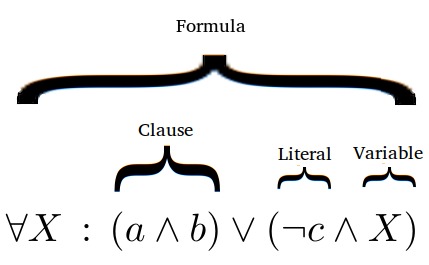
The parts of a logical formula, which could be input data, a constraint, or the output model.
The output of a call to an ILP system (what is induced by the learning algorithm) takes several names: a ‘theory’, a ‘hypothesis’, a ‘program’, a ‘concept’, or a ‘model’ (in the machine learning sense, and not the logical sense of a truth-value interpretation).
ILP is a collection of methods, rather than one technique or even family of algorithms, due to the many systems not based on Prolog-like inference, and the many nonsymbolic ILP systems. Our working criterion is just that the output of an ‘ILP’ system should be a logic program.
How it works
In the classic setting, the examples \(E\) are labelled with a binary class: positive examples \(E^+\) and negative examples \(E^-\). An ILP system searches a hypothesis space \(\mathcal{H}\) until a program \(h\) is found such that \(B \land h \models E^+\), and such that \(\forall e\in E^- \, B\land h \not\models e\). In practice this is weakened in two ways: firstly by heuristic scoring, so that most positives and few negatives are covered by \(h\); and secondly by using \(\theta\)-subsumption rather than normal (undecidable) FOL entailment. \(h\) is then a relational description, in terms of \(B\), of some concept common to the positive examples and absent from the negatives.
The normal ILP setting assumes that atoms are either true or false, and that hypotheses have a binary domain. Thus the first ILP designs produced only binary classifiers. But ‘upgraded’ (relational)\citep{laer} forms of many propositional ML techniques have been developed: multi-class classification \citep{clark}, regression with decision trees \citep{kramer-tree}, clustering \citep{brugh}, and even visual object classification \citep{plane}. This bivalence also entails the inability of early, exact ILP systems to handle ambiguous data.
We can view ILP as a search of the ‘subsumption lattice’, the graph that results from partially ordering hypotheses in \(\mathcal{H}\) from most general (\(\mathrm{true} \to E^+\)) to most specific (the bottom clause \(\bot\), a conjunction of evaluated predicates).
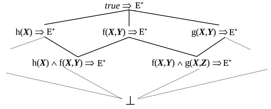
A subsumption lattice to search.
The lattice gives us two obvious approaches to hypothesis discovery in ILP:
‘bottom-up’ search, starting from an initially long clause (i.e. the feature values of individual examples), finds a specific clause to generalise from, and drops or abstracts away literals until a minimally general hypothesis that covers \(E^+\) is found. This specific-to-general search direction is the default approach in the classic ILP systems Progol and Aleph.
‘top-down’ search proceeds from a short clause (for instance, the empty implication
true, and adds literals to it until the expression becomes too specific to cover the examples. This might involve generating candidate clauses from a template, then testing these clauses against \(E\), branching through the lattice when violations are found. This general-to-specific approach is used in Metagol and \(\partial\)ILP.
The expressive power of (even subsets of) first-order logic leads to ILP’s computational complexity: the resulting combinatorial search over large discrete spaces is a notably difficult problem: it’s in \(NP^{NP}\). As a result, various forms of heuristic scoring are used to guide and prune the search.
Table 1 relates the various biases of ILP and DL. For instance, we can draw an analogy between the ‘program template’ that constrains an ILP hypothesis space and the architecture of a neural network; both constrain the hypothesis space and, until recently, both have been entirely handcrafted, though recent results in neural architecture search promise automation of bias provision. Divide inductive bias into
- language bias (hypothesis space restriction),
- procedural bias (how the search is ordered; also called ‘search bias’), and
- simplicity bias (how overfitting is prevented).
I don’t know the standard term for the many ways to bias an ILP run (mode declarations, program templates, meta-rules). So I’ll call them user-supplied constraints (UCs).
| Learning property | ILP | DL |
| Language bias | Program templates | NN architecture |
| Procedural bias | Various: classic search algos | N/A |
| Simplicity bias | Bound on program length | It's controversial |
| Search procedure | Local search for subsumption | Local search over gradients |
| Automated language bias? | No | Sometimes |
Example ILP algorithms
Generic algorithm: ILP as two-part search
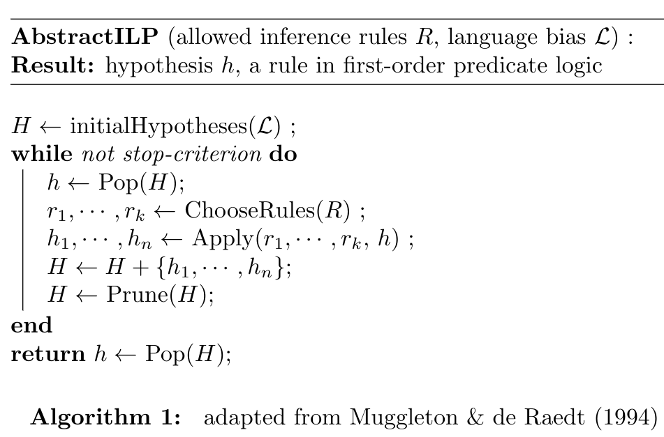
At this level of abstraction (which overlooks the data, even), we see the structure and parameters of ILP in general:
- `initialHypotheses`: defines the hypothesis space. High-performance ILP systems generally begin with only one hypothesis in this queue \(B \land E^+\).
- `stop-criterion`. Terminating condition. Examples include: finding a strict solution; meeting some threshold on the statistical significance of the heuristic score of a hypothesis.
- `Pop`: which hypothesis to try next. This is half of the search procedure. It can proceed by simple classical search, e.g. LIFO (breadth-first) or FIFO (depth-first) or priority queue (best-first), or by heuristics (see `Prune`).
- `ChooseRules` and `Apply`: determines which inference rules to use on \(H\), for instance absorption, addClause, dropNegativeLiteral. These are generally syntactic modifications of \(h\), and yields a set of derived hypotheses \(\{ h_1 \cdots h_n\}\).
- `Prune`: which candidate hypotheses to delete from \(H\); the other half of the search. We score the hypotheses, for instance using estimated probabilities \(p(H | B\land E)\). (Note that, in an exact system, generalisation and specialisation allow us to simultaneously assign \(p = 0\) to all specialisations of hypotheses that fail to entail a positive, and \(p=0\) to all generalisations of hypotheses \( \land \,\mathrm{example}\, e^- \) that entail the empty clause.) An alternative score is the minimum compression length of \(h\).
LaTeX
\KwResult{hypothesis `\(h`\(, a rule in first-order predicate logic} \smallskip \hline \vspace{\baselineskip} % `\(H \leftarrow`\( initialHypotheses(`\(\mathcal{L}`\() \; \While{not \text{stop-criterion}} { `\(h \leftarrow`\( Pop`\((H)`\(\; `\(r_1, \cdots, r_k \leftarrow`\( ChooseRules(`\(R`\() \; `\(h_1, \cdots, h_n \leftarrow`\( Apply(`\(r_1, \cdots, r_k, \, h`\() \; `\(H \leftarrow H + \{ h_1, \cdots, h_n \}`\(\; `\(H \leftarrow`\( Prune(`\(H`\()\; } \textbf{return} `\(h \leftarrow`\( Pop`\((H)`\(\; \smallskip \vspace{\baselineskip} % \caption{\, adapted from Muggleton \& de Raedt (1994) \citep{mugg94-review}} \end{algorithm} \[\] At this level of abstraction (which overlooks the data, even), we see the structure and parameters of ILP in general: %it comprises a hypothesis search subroutine, and a clause selection (heuristic scoring) subroutine. \begin{itemize} \item `initialHypotheses}: defines the hypothesis space. High-performance ILP systems generally begin with only one hypothesis in this queue (`\(B \land E^+)`\(. \item `stop-criterion}. Terminating condition. Examples include: finding a strict solution; meeting some threshold on the statistical significance of the heuristic score of a hypothesis. \item `Pop}: which hypothesis to try next. This is half of the search procedure. It can proceed by simple classical search, e.g. LIFO (breadth-first) or FIFO (depth-first) or priority queue (best-first), or by heuristics (see `Prune}). \item `ChooseRules} and `Apply}: determines which inference rules to use on `\(H`\(, for instance absorption, addClause, dropNegativeLiteral. These are generally syntactic modifications of `\(h`\(, and yields a set of derived hypotheses `\(\{ h_1 \cdots h_n\}`\(. % \item `Prune}: which candidate hypotheses to delete from `\(H`\(; the other half of the search. We score the hypotheses, for instance using estimated probabilities `\(p(H | B\land E)`\(. (Note that, in an exact system, generalisation and specialisation allow us to simultaneously assign `\(p = 0`\( to all specialisations of hypotheses that fail to entail a positive, and `\(p=0`\( to all generalisations of hypotheses `\(\land `\( example `\(e^-`\( that entail the empty clause.) An alternative score is the minimum compression length of `\(h`\(. \end{itemize}
Top-down search: The First-Order Inductive Learner

LaTeX
\qquad\qquad positive examples $E^+$,
\qquad\qquad negative examples $E^-$) :
\KwResult{hypothesis $h$, a rule in first-order predicate logic} \smallskip \hline \vspace{\baselineskip} %TODO literals = {predicates in the problem statement and their negatives, (in)equality b/w bound variables} $h \leftarrow \emptyset$
\While{$E^+$ not empty} { $\mathrm{clause} \leftarrow \mathrm{LearnNewClause}(E^+, E^-, h)$
candidateTheory $\leftarrow B\land h\land \mathrm{clause}$
coveredPositives $\leftarrow \{e\in E^+ \colon $ candidateTheory $\vdash e\}$
$E^+ \leftarrow E^+ \,\setminus $ coveredPositives
$h \leftarrow h \cup \{\mathrm{clause}\}$
} \textbf{return} $h$
\end{algorithm} \vspace{\baselineskip} \begin{algorithm}[H] \hline\smallskip \textbf{LearnNewClause}($E^+, E^-, h$) : \smallskip\hline \smallskip\smallskip % $\mathrm{clause} \leftarrow \emptyset$
\While{$E^-$ not empty}{ $\mathrm{bestLiteral} \leftarrow \argmax\limits_{l} \,\, \mathrm{Gain}(\mathrm{clause}, l, E^+, E^-)$
$\mathrm{clause} \leftarrow \mathrm{clause} \cup \{\mathrm{bestLiteral}\}$
candidateTheory $\leftarrow B\land h\land \mathrm{clause}$
coveredNegatives $\leftarrow \{e\in E^- \colon $ candidateTheory $\vdash e\}$
$E^- \leftarrow E^- \,\,\setminus$ coveredNegatives
} \textbf{return} clause
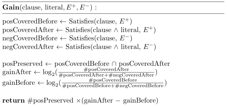
\vspace{\baselineskip} \vspace{\baselineskip} % % % \hline\smallskip \textbf{Gain}(clause$, $ literal$, E^+, E^-$) :
\smallskip\hline \smallskip\smallskip % posCoveredBefore $\leftarrow$ Satisfies(clause, $E^+$)
posCoveredAfter $\leftarrow$ Satisfies(clause $\land$ literal, $E^+$)
negCoveredBefore $\leftarrow$ Satisfies(clause, $E^-$)
negCoveredAfter $\leftarrow$ Satisfies(clause $\land$ literal, $E^-$)
\vspace{\baselineskip} posPreserved $\leftarrow$ posCoveredBefore $\cap$ posCoveredAfter
gainAfter $\leftarrow \log_2 (\frac{\#\mathrm{posCoveredAfter}} {\#\mathrm{posCoveredAfter} + \#\mathrm{negCoveredAfter}})$
% gainBefore $\leftarrow \log_2 (\frac{\#\mathrm{posCoveredBefore}} {\#\mathrm{posCoveredBefore} + \#\mathrm{negCoveredBefore}})$
\vspace{\baselineskip} \textbf{return} \#posPreserved $\times ($gainAfter $-$ gainBefore$)$
% % \vspace{\baselineskip} \vspace{\baselineskip} \caption{ \,adaptation of FOIL \citep{foil}\citep{vinay} with gain heuristic} \end{algorithm} %This is also known as a 'greedy cover set' algorithm. % greedy covering heuristic
Bottom-up search: The default Aleph algorithm
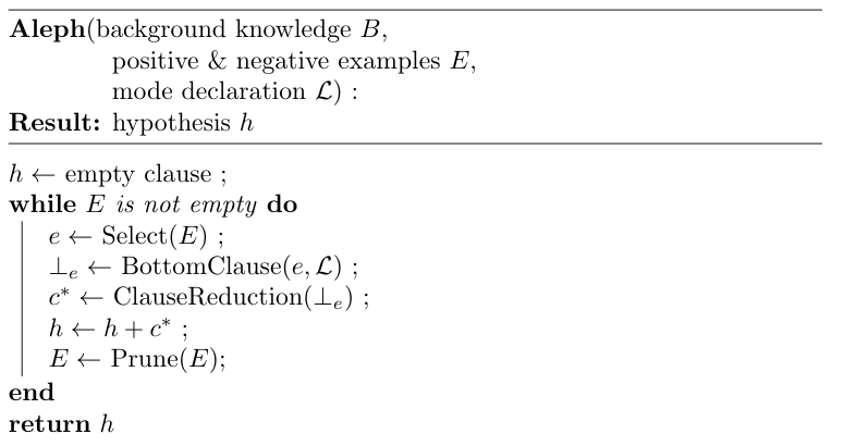
LaTeX
\qquad\qquad positive \& negative examples $E$,
\qquad\qquad mode declaration $\mathcal{L}$) :
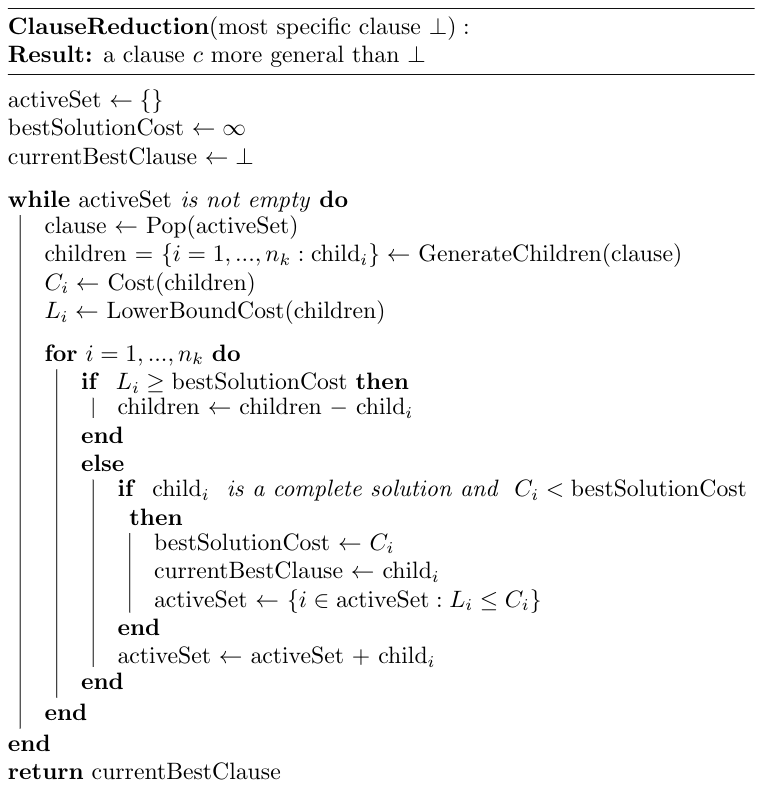
\KwResult{hypothesis $h$} \smallskip\hline \smallskip\smallskip % $h \leftarrow $ empty clause \; \While{$E$ is not empty}{ $e \leftarrow$ Select$(E)$ \; $\bot_e \leftarrow$ BottomClause$(e, \mathcal{L})$ \; $c^* \leftarrow $ ClauseReduction$(\bot_e)$ \; $h \leftarrow h + c^*$ \; $E \leftarrow$ Prune$(E)$\; } \textbf{return} $h$ % \vspace{\baselineskip} \hline\smallskip \textbf{ClauseReduction}(most specific clause \bot) :
\KwResult{a clause $c$ more general than $\bot$} \smallskip \hline \smallskip\smallskip % activeSet $\leftarrow \{ \nullset \}$
bestSolutionCost $\leftarrow \infty$
currentBestClause $\leftarrow \bot$
\smallskip\smallskip \While{$\mathrm{activeSet}$ is not empty} { clause $\leftarrow$ Pop$($activeSet$)$
children = $\{ i=1,...,n_k : \mathrm{child}_i \} \leftarrow$ GenerateChildren$($clause$)$
$C_i \leftarrow$ Cost$($children$)$
$L_i \leftarrow$ LowerBoundCost$($children$)$
% \smallskip\smallskip % \For{$i = 1,..., n_k$} {
\If{ $L_i \geq \mathrm{bestSolutionCost}$} { children $\leftarrow$ children $-$ child$_i$
}
\Else {
\If{ $\mathrm{child}_i$ \text{ is a complete solution and } $C_i < \mathrm{bestSolutionCost}$ } {
bestSolutionCost $\leftarrow$ $C_i$
currentBestClause $\leftarrow$ child$_i$
activeSet $\leftarrow$ $\{ i \in \mathrm{activeSet} : L_i \leq C_i \}$
}
activeSet $\leftarrow$ activeSet $+$ child$_i$
} }
}
\textbf{return} currentBestClause % \vspace{\baselineskip} \caption{\,Adapted from Srinivasan (1999) \citep{aleph}.} \end{algorithm} \begin{itemize} % \item \texttt{Select}: pick an example $e$ to be generalised. \item \texttt{BottomClause}: 'saturate' the example - find the most specific clause that both entails $e$ and obeys the mode declaration (that is, the specified language bias). The procedure is from \citep{progol}. \item \texttt{ClauseReduction}: search for a subset (or derived subset) of the literals in $\bot_e$ with the best score, arg max$_c\,$ Score$(\bot_e)$. This is a branch-and-bound algorithm, and returns a search tree with clauses for nodes. As standard, this is the gain in accuracy of adding $c$ to $h$. A 'good' clause is defined by hyperparameters: a maximum clause length, a minimum accuracy, a minimum 'child weight' (i.e. a threshold number of positive examples covered by $c$ before $c$ can be selected). \item \texttt{Prune}: remove examples (and background) made redundant under the new hypothesis $h$. Unlike Algorithm 1, this prunes the \textit{examples} rather than the candidate hypotheses. % \end{itemize}
Classifying ILP Systems
- Order of hypotheses: does it allow first-order logic or higher-order logics in the representation of inputs, intermediates, and outputs?
- Target language: Almost all ILP systems induce Prolog programs; however recent systems use other target languages, for instance Datalog (less expressive than Prolog) or answer-set programming\citep{ilasp} (more expressive).
- Search strategy: whether the search is conducted top-down (that is, from general to specific) or bottom-up (starting with an example and generalising it), or whether both are used (as in 'theory revision').
- Exact or probabilistic search: does the search include stochastic steps?
- Noise handling: how are mislabeled examples or other corrupt data-points handled? An implementation detail, this can involve restricting specialisation in top-down search; allowing some negatives to be covered by a clause; or by using a neural network to preprocess data. % metagol is a kind of bootstrap scoring
- Inference engine: Almost all ILP systems are meta-interpreters running on Prolog. More recent systems attempt to replace symbolic inference with latent embeddings in a structured neural network or some other differentiable structure, for instance the differentiable deduction (\(\partial D\)) of \(\partial\mathrm{ILP}\).
- Predicate invention: can the system induce new background assumptions during learning?
| System | Order | Target | Search | Exact | Noise | Engine | Invent |
| FOIL | First | Prolog | Top-down | Yes | None | Prolog | No |
| Progol | First | Prolog | Top-down | Yes | Bounded | Prolog | No |
| Aleph | First | Prolog | Bottom-up | Both | Bounded | Prolog | No |
| Metagol | Higher | Datalog/ASP | Top-down | Yes | Scoring | Prolog | Yes |
| \(\partial\)ILP | First | Datalog | Top-down | No | ANN | $$\partial D$$ | Yes |
Theoretical bounds
One of the dirty secrets of computer science is that formal proofs about computability and complexity are often practically useless. (Neural networks trained with RL have dented PSPACE-hard problems like playing Go, and more generally worst-case theories like Rademacher complexity overestimate the actual generalisation error of neural networks.) But even then, still interesting.
How do we beat complexity results?
* Giving up optimality: If we assume diminishing returns to optimisation, a suboptimal solution within a fixed margin (\(\epsilon\)) of the optimal one may be exponentially (\(\exp{1/\epsilon}\)) faster to find.
* Giving up correctness: Randomisation can reduce hardness significantly. Also, the cost of giving up (necessary) correctness can be offset in some cases by several independent runs of the algorithm that make the probability of an error vanish exponentially in the number of runs.
* Giving up generalisation: A narrower algorithm may be faster and still useful in most cases.
[Section forthcoming]
Expressivity
Computability
Complexity
Generalisation
Limitations
Naivety about noise and ambiguity.
In simple concept learners, a single mislabelled example can prevent learning entirely. However, progress has been made in handling noise and ambiguity: first, the low-hanging fruit of detecting mutual inconsistency in data (by deriving contradictions); and second limiting how far a top-down specialisation should go, when noise is assumed to be present. Further, the use of learned hypotheses for transfer learning between runs of ILP is limited by the noise a given learned program is likely to have picked up: current systems assume that background knowledge (like a transferred program) is certain.
Large resource requirements.
We discussed the terseness of ILP outputs as a virtue, but it’s equally true that present systems cannot learn large theories given practical compute. The space complexity of admissible search (that is, algorithms guaranteed to yield an optimum) is exponential in hypothesis length for some systems like Progol. For this reason, predicate invention is limited even in state-of-the-art systems to, at most, dyadic predicates. This appears related to the expressivity of FOL.
Handcrafting task-specific inductive biases.
Almost all ILP systems use user-supplied constraints to generate the candidate clauses that form predicates (for instance ‘mode declarations’ in Progol and Aleph, meta-rules in Metagol, or rule templates in \(\partial\)ILP). In some sense these are just hyperparameters, as found in most ML systems. But templates can be enormously informative, up to and including specifying which predicates to use in the head or body of \(h\), the quantifier of each argument in the predicate, which arguments are to be treated inputs and outputs, and and so on. Often unavoidable for performance reasons, templates risk pruning unexpected solutions, involve a good deal of expert human labour, and lead to brittle systems which may not learn the problem structure, so much as they are passed it to begin with.
This is an open problem, though recent work has looked at selecting or compressing given templates. The \(\partial\)ILP authors also report an experiment with generating templates, but the authors note that at least their brute-force approach is straightforwardly and permanently infeasible\citep{diffilp}.
Usability.
ILP systems remain a tool for researchers, and specialists at that: to our knowledge, no user-friendly system has so far been developed. (The RDM Python wrapper is a partial exception. To some extent this is due to the data representation: somewhat more than a working knowledge of first-order logic and (usually) Prolog are required to input one’s own data. Whether this is a higher barrier than the basic linear algebra required for modern deep learning libraries, or merely a rarer skill in the data science community, would require empirical study. But the effect is the same: ILP seems more difficult to use.
The deep threat to knowledge representation.
The “knowledge representation” programme is challenged by rapid progress in learned representations and end-to-end deep learning in computer vision, natural language processing, and many other fields. Rich Sutton summarises this challenge as “the bitter lesson”: that massively scaling dataset size and model size tends to outperform hand-crafting of features and heuristics by domain experts. This is a ‘limitation’ of ILP insofar as it cannot itself follow suit and take advantage of learned representations to the same degree.
An even more contentious claim: perhaps we shouldn’t expect human-sized steps in advanced machine reasoning. If the bitter lesson holds in general, then expert elicitation is dead.
See also
Thanks to Javi Prieto, Nandi Schoots, and Joar Skalse for many, many comments.